library(knitr)
download.file("https://zenodo.org/records/7681811/files/sachs.zip?download=1",
              "sachs.zip", mode = "wb")
unzip("sachs.zip", files = "Data Files/cd3cd28.csv")
cd3cd28   <- read.csv(file.path("Data Files", "cd3cd28.csv"))
Sachs_mat <- as.matrix(cd3cd28)
n <- nrow(Sachs_mat)6 Cost-Aware Optimized Front-Door Experimental Design
Leopold Mareis 
Mathias Drton
| Resource | Information |
|---|---|
| Data DOI | 10.5281/zenodo.7681811 |
| Git + DOI | Git 10.5281/zenodo.20613058 |
| Paper | arXiv |
| Paper Code | Git 10.5281/zenodo.18960268 |
| Short Description | Demonstration of the optimized experimental design for subsequent causal effect estimation of Mareis and Drton (2026) on the Sachs protein-signalling dataset. |
6.1 Introduction
The Sachs dataset records expression levels provides in human T cells and is accompanied by a validated ground-truth causal DAG recovered through targeted perturbation experiments (Sachs et al. 2005; Kleinegesse, Lawrence, and Chockler 2022). In this notebook, we present the cost-aware experimental design framework of Mareis and Drton (2026) to two estimation problems:
back-door estimation of the direct effect of Mek on Erk, and
front-door estimation of the total causal effect of Mek on Akt.
While sampling, every unit contributes a baseline observation \((x_C, x_t)\); the experimenter then decides whether to additionally measure \(x_M\) and, in the front-door case, \(x_r\). The optimal design assigns unit-specific sampling probabilities \((\pi_1(x_C, x_t),\, \pi_2(x_C, x_t, x_M))\): units with high information-to-cost ratios for \(\beta_{Mt}\) or \(\beta_{rM}\) are measured more intensively, while others are subsampled. This yields a strictly lower asymptotic estimation variance than full measurement at equal total cost.
The following application computes this optimal design and reports the resulting efficiency gains, beginning with the simpler single-stage back-door problem before extending to the two-stage front-door setting.
6.2 Problem: Cost-Aware Causal Effect Estimation
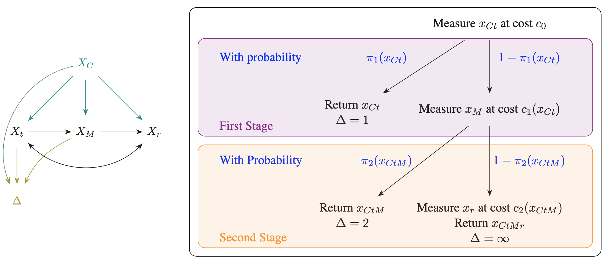
The linear multivariate front-door model comprises confounders \(X_C\), treatment \(X_t\), mediator \(X_M\), and response \(X_r\), related by the structural equation \(X = \beta X + \varepsilon\), where \(\beta\) is lower-triangular and \(\varepsilon\) allows for arbitrary confounding between \(\varepsilon_t\) and \(\varepsilon_r\); see Figure 6.1. Under the front-door condition, requiring every causal path from \(X_t\) to \(X_r\) to pass through \(X_M\), the causal effect reduces to \[\xi = \beta_{rM}\beta_{Mt},\] identified via the two regressions \(X_t \to X_M\) and \(X_M \to X_r\), each adjustable by \(X_C\).
Data collection proceeds in two stages beyond the always-observed baseline \((x_C, x_t)\) at cost \(c_0\). The first stage measures \(x_M\) with probability \(\pi_1(x_C, x_t)\) at cost \(c_1\); the second measures \(x_r\) with probability \(\pi_2(x_C, x_t, x_M)\) at cost \(c_2\). The indicator \(\Delta \in \{1, 2, \infty\}\) records the stage reached. The optimal \((\pi_1^*, \pi_2^*)\) minimizes the asymptotic variance \(\mathrm{Var}_\infty(\hat\xi;\,\pi)\) over regular asymptotically linear (RAL) estimators, subject to \(\mathbb{E}[c_0 + \pi_1 c_1 + \pi_1\pi_2 c_2] = b_0\). The relative efficiency \[\frac{\mathrm{Var}_\infty(\hat\xi;\,\pi^*)}{\mathrm{Var}_\infty(\hat\xi;\,1)\cdot\mathrm{scale}},\] where scale, or oversampling, equalizes total cost, certifies a gain when below 1.
The front-door factorization \(\xi = \beta_{rM}\beta_{Mt}\) decomposes into two regressions: \(\beta_{Mt}\) from \((X_C, X_t, X_M)\), which is a self-contained back-door problem; and \(\beta_{rM}\) from \((X_C, X_t, X_M, X_r)\), the distinctly front-door component. The optimized back-door design presented below applies to any back-door estimation setting, independent of whether a response \(X_r\) is available.
NoteKey insight. Two structural observations motivate cost-aware partial-data designs.
Partial sufficiency. Some estimands do not depend on all data columns: \(\beta_{Mt}\) requires only \((X_C, X_t, X_M)\) and not \(X_r\), while \(\beta_{rM}\) additionally requires \(X_r\). Estimands with partial column support can be recovered from incompletely observed units without bias, so full measurements are not needed for every unit.
Budget reallocation. Under a fixed total budget, skipping expensive later stages reduces the per-sample cost, allowing more units to enter the study. The relative efficiency quantifies the trade-off: whether the variance reduction from additional samples outweighs the information lost from partial observations.
6.3 Sachs Dataset
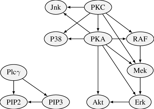
The Sachs dataset (Sachs et al. 2005) records \(n = 853\) simultaneous expression levels of 11 proteins and phospholipids in human T cells under cd3cd28 (CD3/CD28 antibody) stimulation. The ground-truth causal DAG, shown in Figure 6.2, was established through a combination of observational data analysis and targeted perturbation experiments (Sachs et al. 2005; Kleinegesse, Lawrence, and Chockler 2022). For the back-door analysis we use PKA as confounder (\(X_C\)), Mek as treatment (\(X_t\)), and Erk as mediator (\(X_M\)); the front-door analysis additionally uses Akt as response (\(X_r\)).
Kleinegesse, Steven, Andrew R. Lawrence, and Hana Chockler. 2022. “Domain Knowledge in a*-Based Causal Discovery.”
| PKA | Mek | Erk | Akt |
|---|---|---|---|
| 414 | 13.20 | 6.61 | 17.0 |
| 352 | 16.50 | 18.60 | 32.5 |
| 403 | 44.10 | 14.90 | 32.5 |
| 528 | 82.80 | 5.83 | 11.8 |
| 305 | 19.80 | 21.10 | 46.1 |
| 610 | 3.75 | 11.90 | 25.7 |
6.4 Optimized Design for Back-Door Estimation \(\beta_{Mt}\)
Cost-aware back-door estimation of \(\beta_{Mt}\) relies only on \((X_C, X_t, X_M)\). The sampling decision is: observe \((x_C, x_t)\) at cost \(c_0\), then measure \(x_M\) with probability \(\pi_1(x_C, x_t)\) at additional cost \(c_1\).
We apply this methodology with \(X_C = \text{PKA}\), \(X_t = \text{Mek}\), \(X_M = \text{Erk}\), and \(c_0 = 2\), \(c_1 = 1\). In the Sachs ground-truth DAG, PKA blocks all back-door paths from Mek to Erk, satisfying the back-door adjustment criterion.
The companion repository (see resource table) provides implementations for estimate_parameters, compute_moments, compute_oif_variance, compute_expected_cost, and compute_optimal_pi. The analysis estimates parameters from the observed data, evaluates the asymptotic variance under full measurement, and scans over oversampling levels to compute the relative efficiency.
source("functions_back_door.R")set.seed(1234)
data_bd <- data.frame(
C = rep(Inf, n), # Delta
X_t = Sachs_mat[, 2], # Mek
X_M = I(Sachs_mat[, 6, drop = FALSE]), # Erk
X_C = I(Sachs_mat[, 8, drop = FALSE]) # PKA
)
pi1_fun_bd <- function(XCt) rep(1, nrow(XCt))
c1_fun_bd <- function(XCt) rep(1, nrow(XCt))
estimates_bd <- estimate_parameters(data_bd, pi1_fun_bd)
mom_bd <- compute_moments(data_bd, estimates_bd, pi1_fun_bd)
avar_vanilla_bd <- compute_oif_variance(data_bd, estimates_bd, pi1_fun_bd,
pi1 = rep(1, n))
cost_vanilla_bd <- compute_expected_cost(rep(1, n), c0 = 2,
c1_fun_bd(data_bd[, c("X_C", "X_t")]),
mom_bd$Weight_2inf)
scales_bd <- seq(1.05, 1.25, by = 0.05)
rel_effs_bd <- vapply(scales_bd, function(s) {
opt <- compute_optimal_pi(data_bd, estimates_bd,
c0 = 2, c1_fun = c1_fun_bd,
b0 = cost_vanilla_bd / s,
pi1_0_fun = pi1_fun_bd, n_sub = 10000)
avar_opt <- compute_oif_variance(data_bd, estimates_bd, pi1_fun_bd,
pi1 = opt$pi1_star)
avar_opt / avar_vanilla_bd / s
}, numeric(1))
scale_bd <- 1.15
rel_eff_bd <- rel_effs_bd[3]| Scale | Relative Efficiency |
|---|---|
| 1.05 | 0.9540 |
| 1.10 | 0.9211 |
| 1.15 | 0.9064 |
| 1.20 | 0.9161 |
| 1.25 | 0.9588 |
The table confirms that the partial sampling design achieves a variance reduction at every oversampling level considered. At \(15%\) oversampling, it attains a relative efficiency of 0.9064, a 9.4% gain over uniform full measurement at equal total budget.
6.5 Optimized Design for Front-Door Estimation of \(\xi\)
The back-door analysis estimated \(\beta_{Mt}\), the direct effect of Mek on Erk, using only \((X_C, X_t, X_M)\). The front-door setting extends this to the total causal effect \(\xi = \beta_{rM}\beta_{Mt}\) of Mek on Akt, which additionally requires measuring the response \(X_r = \text{Akt}\). Since PKA has a direct edge to Akt in the Sachs DAG, the pair (Mek, Akt) is confounded and the front-door path through Erk is the identification strategy; see Figure 6.2.
The two-stage design introduces a second propensity \(\pi_2(x_C, x_t, x_M)\) governing whether Akt is measured after Erk. The joint optimization of \((\pi_1^*, \pi_2^*)\) balances the leverage of treatment residuals against mediator residuals under the combined budget constraint, with \(X_C = \text{PKA}\), \(X_t = \text{Mek}\), \(X_M = \text{Erk}\), \(X_r = \text{Akt}\), and custom costs \(c_0 = 2\), \(c_1 = c_2 = 1\).
source("functions.R")# Column indices: 2=Mek, 6=Erk, 7=Akt, 8=PKA
pi1_fun <- function(XCt) rep(1, nrow(XCt)) # baseline: full measurement
pi2_fun <- function(XCtM) rep(1, nrow(XCtM))
c1_fun <- function(XCt) rep(1, nrow(XCt)) # unit cost per stage
c2_fun <- function(XCtM) rep(1, nrow(XCtM))
set.seed(1234)
data_fd <- data.frame(
C = rep(Inf, n), # Delta
X_t = Sachs_mat[, 2], # Mek
X_M = I(Sachs_mat[, 6, drop = FALSE]), # Erk
X_r = Sachs_mat[, 7], # Akt
X_C = I(Sachs_mat[, 8, drop = FALSE]) # PKA
)
# Estimate β_tC, β_Mt, β_MB, β_rM via nested weighted regression
estimates_fd <- estimate_parameters(data_fd, pi1_fun, pi2_fun)
beta_Mt_hat <- as.numeric(estimates_fd$beta_Mt)
beta_rM_hat <- as.numeric(estimates_fd$beta_rM)beta_Mt (Mek -> Erk): -0.0299 (1-unit increase in Mek raises Erk by -0.0299 units)beta_rM (Erk -> Akt): 1.3627 (1-unit increase in Erk raises Akt by 1.3627 units)Causal effect: xi = beta_rM * beta_Mt = 1.3627 * -0.0299 = -0.0407# Asymptotic variance under full measurement (pi = 1)
mom_fd <- compute_moments(data_fd, estimates_fd, pi1_fun, pi2_fun)
avar_vanilla_fd <- compute_oif_variance(data_fd, estimates_fd, pi1_fun, pi2_fun,
pi1 = rep(1, n), pi2 = rep(1, n))
cost_vanilla_fd <- compute_expected_cost(rep(1, n), rep(1, n), c0 = 2,
c1_fun(data_fd[, c("X_C", "X_t")]),
c2_fun(data_fd[, c("X_C", "X_t", "X_M")]),
mom_fd$Weight_2inf)
# Optimal propensity (pi_1*, pi_2*) at 54% oversampling budget
scale_fd <- 1.54
opt_fd <- compute_optimal_pi(data_fd, estimates_fd,
c0 = 2, c1_fun = c1_fun, c2_fun = c2_fun,
b0 = cost_vanilla_fd / scale_fd,
pi1_0_fun = pi1_fun, pi2_0_fun = pi2_fun,
n_sub = 10000)
# Asymptotic variance under optimal design
avar_opt_fd <- compute_oif_variance(data_fd, estimates_fd, pi1_fun, pi2_fun,
pi1 = opt_fd$pi12_star[, 1],
pi2 = opt_fd$pi12_star[, 2])
rel_eff_fd <- avar_opt_fd / avar_vanilla_fd / scale_fdFront-door | scale = 1.54 | relative efficiency = 0.6802The relative efficiency of 0.6802 at 54% oversampling corresponds to a 32% variance reduction. The two-stage propensity achieves this by exploiting both the treatment residual (informative for \(\hat\beta_{Mt}\)) and the mediator residual (informative for \(\hat\beta_{rM}\)) to direct measurements selectively across the two stages.
6.6 Summary
Both designs achieve strict efficiency gains at the reported oversampling levels. The larger front-door gain reflects the additional design flexibility available when both \(\beta_{Mt}\) and \(\beta_{rM}\) are targeted through the two-stage propensity.
| Problem | Objective | Scale | Relative Efficiency |
|---|---|---|---|
| Back-door | Direct effect of Mek on Erk | 1.15 | 0.9064 |
| Front-door | Causal effect of Mek on Akt | 1.54 | 0.6802 |
Citing this Notebook
Please cite Mareis and Drton (2026). When using the Sachs dataset, please cite Sachs et al. (2005).
Mareis, Leopold, and Mathias Drton. 2026. “Cost-Aware Optimized Front-Door Experimental Design.”
Sachs, Karen, Omar Perez, Dana Pe’er, Douglas A Lauffenburger, and Garry P Nolan. 2005. “Causal Protein-Signaling Networks Derived from Multiparameter Single-Cell Data.” Science 308 (5721): 523–29.
Additional Information
License Information: Please follow the above DOIs for license information of data and code.
Contact: If you have suggestions, feel free to create an issue or contact the authors.