using OscarLeopold Mareis 
Anthony Della Vecchia
Bejamin Hollering
Mathias Drton
| Resource | Information |
|---|---|
| Git + DOI | Git Zenodo.18709429 |
| Short Description | This notebook demonstrates the computational algebraic procedure in OSCAR to determine the identifiability of model parameters in linear graphical models. |
Let \(\Lambda \in \mathbb{R}^{d\times d}\) be a strictly upper-triangular design matrix and let \(\varepsilon \sim P_\varepsilon\) be a centered random vector with positive definite covariance matrix \(\Omega \in \mathbb{R}^{d\times d}\). A random vector \(X\) follows a linear structural equation model (SEM) if it satisfies \[ X = \Lambda^\top X + \varepsilon. \] The induced covariance matrix on a dataset \((X^{i})_{i \in [n]}\) takes the form \[\Sigma := Cov(X) = (Id - \Lambda)^{-T} \Omega (Id - \Lambda)^{-1}. \] These equations define polynomial relations among the observed covariance matrix \(\Sigma\) and the model parameters \((\Lambda, \Omega)\). They may be used both to assess compatibility of a proposed model class with data and to identify model parameters from second-order moments.
Consider the four-variate SEM \[ \begin{pmatrix} X_1 \\ X_2 \\ X_3 \\ X_4 \end{pmatrix} = \begin{pmatrix} 0 & 0 & 0 & 0 \\ 0 & 0 & 0 & 0 \\ \lambda_{12} & \lambda_{13} & 0 & 0 \\ 0 & 0 & \lambda_{34} & 0 \end{pmatrix} \begin{pmatrix} X_1 \\ X_2 \\ X_3 \\ X_4 \end{pmatrix} + \begin{pmatrix} \varepsilon_1 \\ \varepsilon_2 \\ \varepsilon_3 \\ \varepsilon_4 \end{pmatrix}, \quad Cov(\varepsilon) = \begin{pmatrix} \omega_{11} & 0 & 0 & 0 \\ 0 & \omega_{22} & \omega_{23} & 0 \\ 0 & \omega_{23} & \omega_{33} &\omega_{34} \\ 0 & 0 & \omega_{34} & \omega_{44} \end{pmatrix}.\] This random vector satisfies Markov properties encoding conditional independencies with respect to the following acyclic directed mixed graph (ADMG) \(\mathcal{G}\):
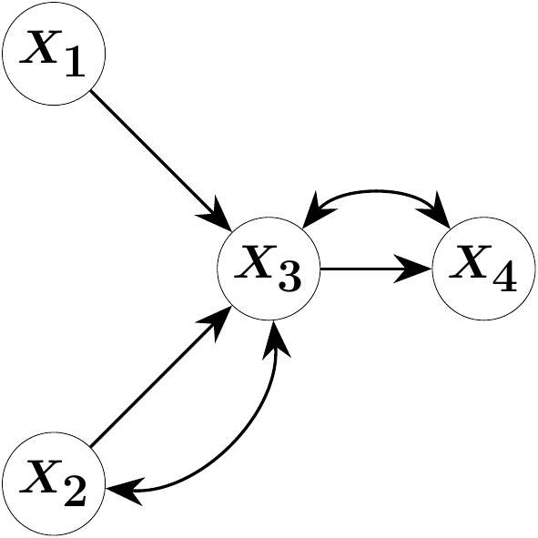
The direct effects \(\lambda_{12}\), \(\lambda_{13}\) and \(\lambda_{34}\) correspond to edges in \(\mathcal{G}\) and constitute the parameters of primary interest. In applications, such direct effects may model, for instance, the efficacy of a medical treatment, the impact of an institutional policy, or the influence of machine settings on manufacturing quality. The graph \(\mathcal{G}\) may be specified by domain experts or inferred via statistical structure learning, after which the corresponding model parameters are to be estimated.
Generic identifiability of model parameters may be assessed via the sufficient but not necessary Half-Trek Criterion (Foygel, Draisma, and Drton (2012)). We describe a computational algebraic approach that is both necessary and sufficient, thereby closing this theoretical gap. All symbolic computations are performed in the Julia package OSCAR (“OSCAR – Open Source Computer Algebra Research System, Version 1.7.0” (2026)).
using OscarThe covariance relation \(\Sigma = (Id - \Lambda)^{-T} \Omega (Id - \Lambda)^{-1}\) defines a polynomial map from the parameter space \((\Lambda,\Omega)\) into the space of symmetric matrices. The model ideal \(\mathcal{I}\) is the linear space in the polynomial ring \(\mathbb{Q}[\Lambda,\Omega,\Sigma]\) generated (spanned) by the relations \[(- (Id - \Lambda^\top)^{-T} \Omega (Id - \Lambda)^{-1})_{ij} - \Sigma_{ij} = 0 \quad \forall i,j \in [d].\] Its zero set is the model variety \(\mathcal{V(I)}\), consisting of all triplets \((\Lambda,\Omega,\Sigma)\) consistent with the postulated statistical model. In the implementation below, the ideal is constructed in a joint polynomial ring over the entries of \(\Lambda\) (denoted l[i,j]), \(\Omega\) (denoted w[i,j]), and \(\Sigma\) (denoted s[i,j]).
function identify_parameters(M::GraphicalModel,
                             return_elimination_ideal = false,
                             return_ideal = false)

  # get graph data from the model
  G = graph(M)
  if typeof(G) === Oscar.MixedGraph
    E = edges(G, Directed)
  else
    E = edges(G)
  end

  # get rings and parametrization
  S, s = model_ring(M)
  R, t = parameter_ring(M)
  phi = parametrization(M)

  # setup the elimination ideal
  elim_ring, elim_gens = polynomial_ring(coefficient_ring(R), vcat(symbols(R), symbols(S)))
  inject_R = hom(R, elim_ring, elim_gens[1:ngens(R)])
  inject_S = hom(S, elim_ring, elim_gens[ngens(R) + 1:ngens(elim_ring)])
  I = ideal([
    inject_S(s) * inject_R(denominator(phi(s))) - inject_R(numerator(phi(s))) for s in gens(S)
  ])
  if return_ideal
    return I
  end

  # eliminate
  out = Dict()
  for e in E
    l = t[e]
    other_params = [inject_R(i) for i in values(t) if i != l]
    J = eliminate(I, other_params)
    if return_elimination_ideal
      out[e] = J
    else
      out[e] = contains_linear_poly(J, inject_R(l), ngens(R))
    end
  end

  return out
end

function print_dictionary(out::Dict{Any, Any})
    for (i, edge) in enumerate(keys(out))
        println(edge)
        show(stdout, "text/plain", out[edge])
        println()
        if i < length(out)
            println()
        end
    end
end
directed_edges = [[1, 3], [2, 3], [3, 4]]
bidirected_edges = [[2, 3], [3, 4]]
graph_admg = graph_from_edges(Mixed, directed_edges, bidirected_edges)
model_admg = gaussian_graphical_model(graph_admg)
generators_ideal_admg = identify_parameters(model_admg, false, true)
display(generators_ideal_admg)Ideal generated by
-w[1] + s[1, 1]
s[1, 2]
-l[1, 3]*w[1] + s[1, 3]
-l[1, 3]*l[3, 4]*w[1] + s[1, 4]
-w[2] + s[2, 2]
-l[2, 3]*w[2] - w[3, 2] + s[2, 3]
-l[2, 3]*l[3, 4]*w[2] - l[3, 4]*w[3, 2] + s[2, 4]
-l[1, 3]^2*w[1] - l[2, 3]^2*w[2] - 2*l[2, 3]*w[3, 2] - w[3] + s[3, 3]
-l[1, 3]^2*l[3, 4]*w[1] - l[2, 3]^2*l[3, 4]*w[2] - 2*l[2, 3]*l[3, 4]*w[3, 2] - l[3, 4]*w[3] - w[4, 3] + s[3, 4]
-l[1, 3]^2*l[3, 4]^2*w[1] - l[2, 3]^2*l[3, 4]^2*w[2] - 2*l[2, 3]*l[3, 4]^2*w[3, 2] - l[3, 4]^2*w[3] - 2*l[3, 4]*w[4, 3] - w[4] + s[4, 4]In the ADMG example, the second generator encodes that \(X_1\) and \(X_2\) are uncorrelated, imposing a single visible constraint that a positive definite \(4\times 4\) matrix must satisfy to lie in \(\mathcal{V(I)}\). By contrast, the first generator immediately yields the identification formula \(\omega_{11} = \sigma_{11}\) expressing that the error variance of \(X_1\) equals the marginal variance of \(X_1\).
Note that we call the function gaussian_graphical_model although the error might be non-Gaussian. This is fine as it solely provides the necessary covariance relations.
A parameter \(\lambda_{ij}\) is generically identifiable if it is uniquely determined as a rational function of \(\Sigma\) on a Zariski-dense subset of the model variety. By a standard result in algebraic statistics (Sullivant (2023), Proposition 16.1.8), this holds if and only if the elimination ideal \[\mathcal{J}_{\lambda_{ij}} := \mathcal{I} \cap \mathbb{Q}[\lambda_{ij}, \sigma]\] contains a polynomial of the form \[\lambda_{ij} \cdot g_1(\Sigma) - g_2(\Sigma),\] for polynomials \(g_1, g_2\) in the entries of \(\Sigma\) with \(g_1\) not vanishing identically on \(\mathcal{V}(\mathcal{I})\). The elimination ideal \(\mathcal{J}_{\lambda_{ij}}\) is computed by eliminating all parameters other than \(\lambda_{ij}\) from \(\mathcal{I}\) via a Gröbner basis computation with an appropriate elimination ordering, as implemented in the eliminate function of OSCAR. The completeness of the Gröbner basis guarantees that if no such polynomial exists after finite steps in \(\mathcal{J}_{\lambda_{ij}}\), then \(\lambda_{ij}\) is generically nonidentifiable.
elimination_admg = identify_parameters(model_admg, true)
print_dictionary(elimination_admg)
Edge(3, 4)
Ideal generated by
s[1, 2]
-s[1, 3]*s[2, 4] + s[1, 4]*s[2, 3]
l[3, 4]*s[2, 3] - s[2, 4]
l[3, 4]*s[1, 3] - s[1, 4]
Edge(1, 3)
Ideal generated by
s[1, 2]
-s[1, 3]*s[2, 4] + s[1, 4]*s[2, 3]
l[1, 3]*s[1, 1] - s[1, 3]
Edge(2, 3)
Ideal generated by
s[1, 2]
-s[1, 3]*s[2, 4] + s[1, 4]*s[2, 3]Inspecting the generators of \(\mathcal{J}_{\lambda_{34}}\) reveals the additional constraint \(-\sigma_{13}\sigma_{24} + \sigma_{14}\sigma_{23} = 0\) on the space of \(4 \times 4\) covariance matrices. Furthermore, its last two generators yield the formulas \[ \lambda_{34} \cdot \sigma_{23} - \sigma_{24}, \quad \lambda_{34} \cdot \sigma_{13} - \sigma_{14}, \] both of which identify the parameter \(\lambda_{34}\) as a rational function of \(\Sigma\). For \(\lambda_{13}\), no such polynomial exists in the corresponding elimination ideal, confirming generic nonidentifiability. Statistically, this reflects an overparameterization: the directed edge \(2\rightarrow 3\) and the bidirected edge \(2\leftrightarrow 3\) jointly render \(\lambda_{13}\) unrecoverable from second-order moments alone.
The following function contains_linear_poly filters the generators of each elimination ideal for polynomials of the required linear form in \(\lambda_{ij}\), returning one identification formula among potentially many.
function contains_linear_poly(J::MPolyIdeal, l::MPolyRingElem, nparams::Int)

  R = base_ring(J)

  for f in gens(J)
    exps = exponents(f)
    for v in exps
      # check for ideal generator with only one of its monomials containing
      # l and with degree 1
      if v[var_index(l)] == 1 && sum(sum(e[1:nparams]) for e in exps) == 1
        return (true, f)
      end
    end
  end

  return (false, R(0))
end
identification_admg = identify_parameters(model_admg)
print_dictionary(identification_admg)Edge(3, 4)
(true, l[3, 4]*s[2, 3] - s[2, 4])
Edge(1, 3)
(true, l[1, 3]*s[1, 1] - s[1, 3])
Edge(2, 3)
(false, 0)Applying the identification procedure to all directed edges of \(\mathcal{G}\) yields: \(\lambda_{34}\) and \(\lambda_{13}\) are generically identifiable, while \(\lambda_{23}\) is not.
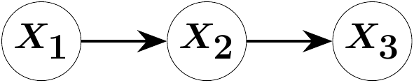
As a consistency check, we apply the same methodology to directed acyclic graphs (DAGs), in which \(\Omega\) is constrained to be diagonal. Suppose the three-variate random vector \(X\) is Markov with respect to the following chain graph:
G = graph_from_edges(Directed, [[1, 2], [2, 3]])
M = gaussian_graphical_model(G)
out = identify_parameters(M)
print_dictionary(out)
Edge(1, 2)
(true, l[1, 2]*s[1, 1] - s[1, 2])
Edge(2, 3)
(true, l[2, 3]*s[2, 2] - s[2, 3])The elimination ideals for both directed edges contain polynomials of the required linear form, yielding the identification formulas \[\lambda_{12} = \frac{\sigma_{12}}{\sigma_{11}}, \quad \lambda_{23} = \frac{\sigma_{23}}{\sigma_{22}},\] corresponding to regression of each variable on its unique parent. Both parameters \(\lambda_{12}\) and \(\lambda_{23}\) are thus generically identifiable, in agreement with the classical theory of graphical models on DAGs.
The algebraic framework described above extends in principle to linear SEMs with cycles, for which \((Id - \Lambda)\) can no longer be permuted to a strictly lower triangular matrix. The construction of the model ideal and the subsequent Gröbner basis elimination proceed without conceptual modification; the polynomial ring and ideal generators are defined identically. This is ensured by clearing rational denominators from the covariance parametrization in identify_parameters. Full implementation support for cyclic graphs is forthcoming in a future release of OSCAR.