# Used packages, only for information.
library(bnlearn)
library(qgraph)
library(igraph)
library(pcalg)
library(huge)
library(zen4R)
library(dplyr)2 ALARM Subgraph Analysis
Stephan Haug 
Oleksandr Zadorozhnyi
| Resource | Information |
|---|---|
| Data | 10.5281/zenodo.14793281 |
| NB | GitHub, 10.5281/zenodo.17238390 |
| Short Description | The text describes the subgraph selection problem in large graphs \(G\). The main objective is to find a smaller subgraph \(S\) that is a meaningful and informative representation of the original graph \(G\). |
2.1 Introduction
Given a large graph \(G = (V, E)\), where \(V\) represents the set of nodes and \(E\) represents the set of edges, the goal is to select a subgraph \(S = (V_s, E_s)\) from G such that S is a meaningful and informative representation of the original graph \(G\). The subgraph selection problem involves finding an optimal or near-optimal subgraph that satisfies certain criteria or objectives.
In the context of graphical modelling the problem of subgraph selection corresponds to the problem of preserving the conditional independence relationship in the subgraph \(S\) which has to be transferred from the underlying graph \(G\).
Furthermore, it is important to be able to evaluate the results of the structure learning algorithms (learned on the data) taking as a ground truth the selected subgraph.
2.1.1 Loading the Data
For our analysis we will need the following packages.
To read files into R hosted on Zenodo, one can use the zen4R package. One starts by setting up the ZenodoManager
zenodo <- ZenodoManager$new()The ALARM dataset is contained in the Zenodo record 10.5281/zenodo.14793281. The record contains two data objects, which can be listed with the following command.
rec <- zenodo$getRecordByDOI("10.5281/zenodo.14793281")
files <- rec$listFiles(pretty = TRUE)
files
filename filesize checksum
alarm.bif alarm.bif 13376 36d1b19ed6a4514e17d2321d1ffb580a
alarm.csv alarm.csv 5661286 0df128ae98e2a899c9de1f27c7c49d4a
download
alarm.bif https://zenodo.org/api/records/14793281/files/alarm.bif/content
alarm.csv https://zenodo.org/api/records/14793281/files/alarm.csv/contentThe file alarm.csv contains the raw data and will be downloaded in the next step using the readr package.
alarm_df <- readr::read_csv(files[2, 4])
alarm_df <- alarm_df |>
  mutate(across(everything(), ~ case_when(
    .x == "FALSE" ~ 0, .x == "TRUE" ~ 1,
    .x == "ZERO" ~ 0, .x == "LOW" ~ 1, .x == "NORMAL" ~ 2,
    .x == "HIGH" ~ 3, .x == "ONESIDED" ~ 3, .x == "ESOPHAGEAL"~  4)))
alarm_df
# A tibble: 20,000 × 37
CVP PCWP HIST TPR BP CO HRBP HREK HRSA PAP SAO2 FIO2 PRSS
<dbl> <dbl> <dbl> <dbl> <dbl> <dbl> <dbl> <dbl> <dbl> <dbl> <dbl> <dbl> <dbl>
1 2 2 0 1 2 3 3 3 3 2 2 1 3
2 2 2 0 2 1 1 3 3 3 2 1 2 3
3 2 3 0 2 2 3 3 3 3 2 1 2 2
4 2 2 0 1 1 3 3 3 3 2 2 2 3
5 2 2 0 1 1 2 3 3 3 2 1 2 1
6 2 2 0 1 2 3 3 3 3 2 1 2 3
7 2 2 0 1 1 3 3 3 3 2 1 1 1
8 2 2 0 2 1 1 3 2 2 1 1 2 3
9 2 1 0 1 1 3 3 3 3 2 1 2 3
10 2 2 0 2 2 3 3 3 3 1 1 2 3
# ℹ 19,990 more rows
# ℹ 24 more variables: ECO2 <dbl>, MINV <dbl>, MVS <dbl>, HYP <dbl>, LVF <dbl>,
# APL <dbl>, ANES <dbl>, PMB <dbl>, INT <dbl>, KINK <dbl>, DISC <dbl>,
# LVV <dbl>, STKV <dbl>, CCHL <dbl>, ERLO <dbl>, HR <dbl>, ERCA <dbl>,
# SHNT <dbl>, PVS <dbl>, ACO2 <dbl>, VALV <dbl>, VLNG <dbl>, VTUB <dbl>,
# VMCH <dbl>The second file in the Zenodo record describes the “true” graph proposed for the ALARM dataset in Scutari and Denis (2021). To read in the bif file, we can use the function read.bif() from the bnlearn package. It creates a bn.fit object, which can be plotted using graphviz.plot().
Scutari, Marco, and Jean-Baptiste Denis. 2021. Bayesian Networks with Examples in R. 2nd ed. Boca Raton: Chapman; Hall.
true_graph <- read.bif(files[1, 4])
graphviz.plot(true_graph, shape = "circle", fontsize = 20)
Loading required namespace: Rgraphviz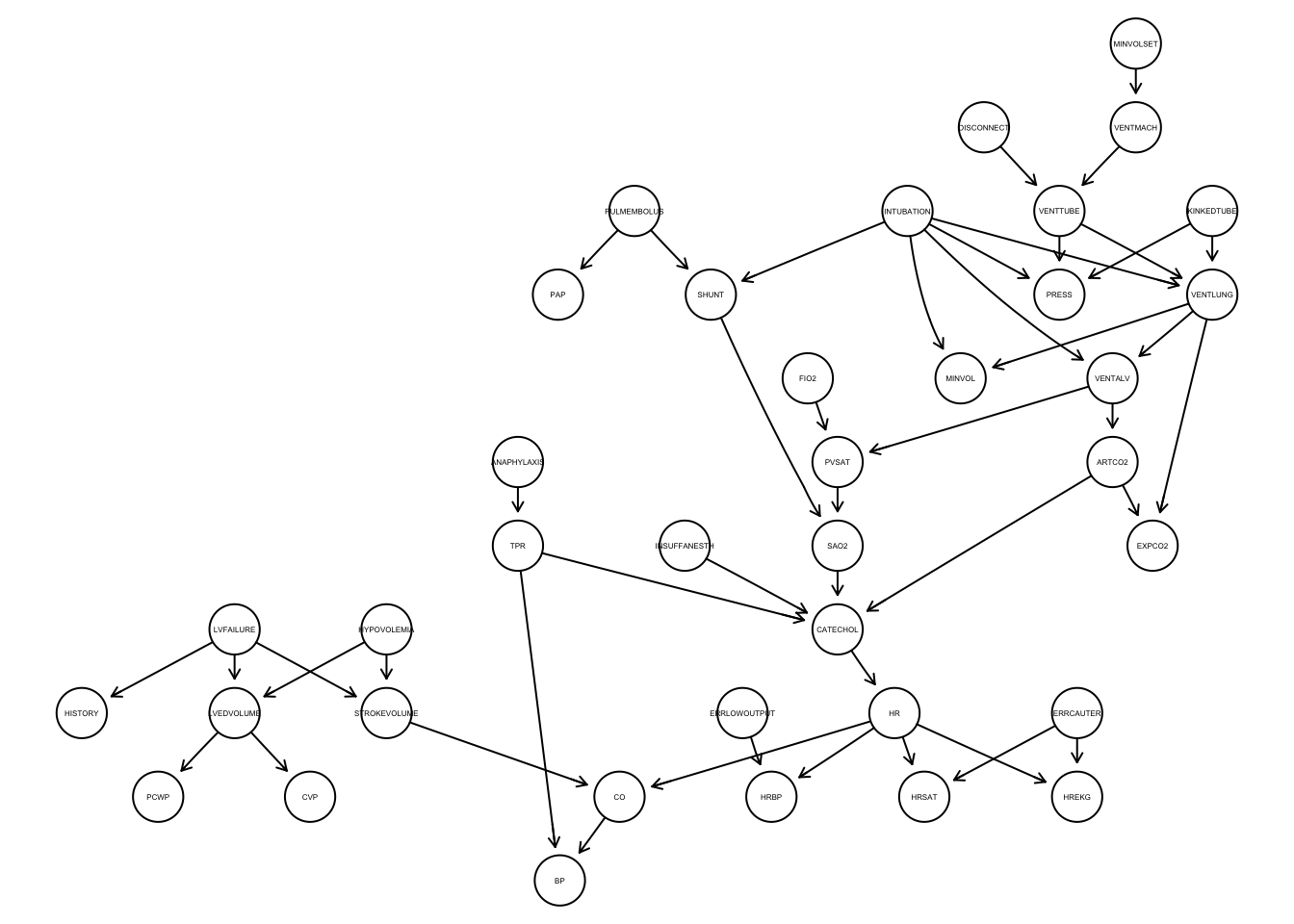
Applying a nonparanormal transformation to standardize the data
alarm_df <- huge.npn(alarm_df)Conducting the nonparanormal (npn) transformation via shrunkun ECDF....done.Defining “true” graph as proposed for the ALARM dataset in bnlearn
# "True" Graph ALARM
dag_alarm = empty.graph(names(alarm))
modelstring(dag_alarm) = paste0("[HIST|LVF][CVP|LVV][PCWP|LVV][HYP][LVV|HYP:LVF]",                    "[LVF][STKV|HYP:LVF][ERLO][HRBP|ERLO:HR][HREK|ERCA:HR][ERCA][HRSA|ERCA:HR]",
"[ANES][APL][TPR|APL][ECO2|ACO2:VLNG][KINK][MINV|INT:VLNG][FIO2]",            "[PVS|FIO2:VALV][SAO2|PVS:SHNT][PAP|PMB][PMB][SHNT|INT:PMB][INT]",              "[PRSS|INT:KINK:VTUB][DISC][MVS][VMCH|MVS][VTUB|DISC:VMCH]",                    "[VLNG|INT:KINK:VTUB][VALV|INT:VLNG][ACO2|VALV][CCHL|ACO2:ANES:SAO2:TPR]",
"[HR|CCHL][CO|HR:STKV][BP|CO:TPR]", sep = "")

qgraph::qgraph(dag_alarm, legend.cex = 0.3,
       asize = 2, edge.color="black", vsize= 4)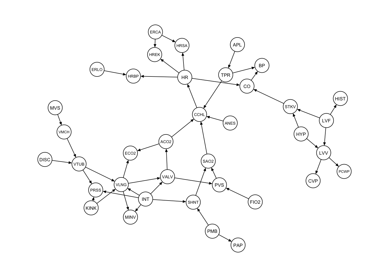
Choosing the nodes to consider in the subgraph selection problem
subgraph_nodes <- c("INT","VALV","LVF","LVV","PCWP","HR","CCHL",
                    "CVP","HYP","HRSA","ERCA")
2.2 Subgraph selection procedures
The first procedure we consider is a simple subsetting of the edges adjacent to the vertices in the subgraph_nodes set. We can accomplish this using the subgraph() function from the bnlearn package.
procedure1 <- bnlearn::subgraph(dag_alarm, subgraph_nodes)
qgraph::qgraph(procedure1, legend.cex = 0.3, asize = 2,
       edge.color = "black", vsize = 5)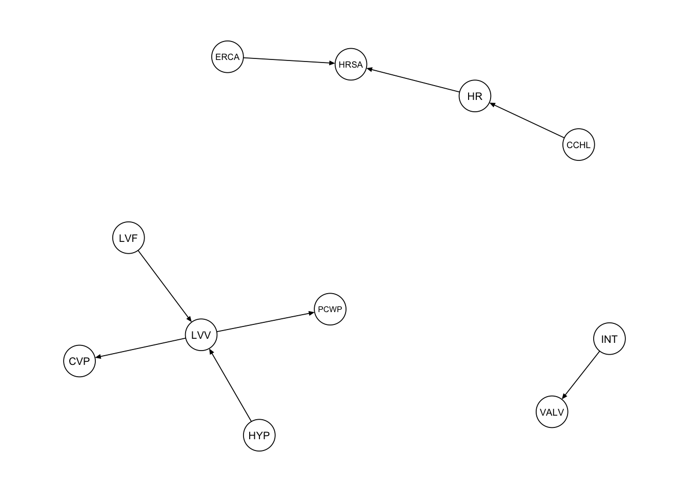
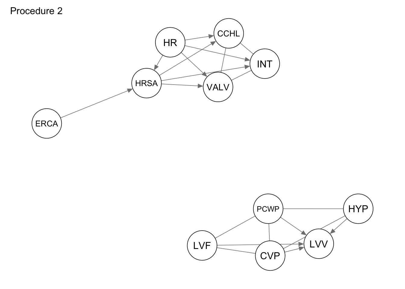
Second procedure selects the subgraph based on the following heuristics:
We are given the ground truth DAG \(G=(V, E)\) with corresponding joint distribution \(\mathsf{P}_V\), and a subset of vertices \(V_{s} \subset V\). The goal is to find the corresponding set of vertices \(E_{s}\) such that the distribution \(\mathsf{P}_{V_s}\) corresponding to \((V_s, E_s)\) does not contradict the structure of the distribution \(P_{V}\).
Let \(G = (V,E)\) be the original directed acyclic graph, and \(P_{V}\) is the joint distribution of random variables from \(V\).
We select two vertices and verify if these vertices are \(d\)-connected given all other vertices in \(V_{s}\). If they are not \(d\)-connected, there is no association (no arrow in any direction). Otherwise, we have an association, but with unknown direction. If one of the directions leads to a cycle in the original graph, we resolve it and keep the other direction, otherwise we keep both directions and then get the CPDAG.
We need to consider all pairs of nodes contained in subgraph_nodes. There exists 2, 55 pairs in total.
The process of checking the \(d\)-connectivity of all pairs of nodes, is implemented in the following function.
extract_subgraph <- function(dag, nodes){
  sg <- bnlearn::subgraph(dag,nodes) # procedure 1 (to be discussed)
  combinations <- combn(nodes,2) # all combinations of 2 distinct nodes in "nodes"
  n <- dim(combinations)[2]
  for (i in 1:n){
    observed <- nodes[nodes!=combinations[1,i] & nodes!=combinations[2,i]] # V'\{v,w}
    if (!is.element(combinations[1,i], nbr(sg, combinations[2,i])) & # check if there exists an edge already
        !bnlearn::dsep(dag,combinations[1,i],combinations[2,i])){ ### check if d-connected
      sg <- set.edge(sg, from = combinations[1,i], to = combinations[2,i]) ### undirected edge in case d-connected
    }
  }
  return(cpdag(sg)) ### to be discussed: return(cpdag(sg))
}
Based on the second procedure we get the following graph.
procedure2 <- extract_subgraph(dag_alarm, subgraph_nodes)
qgraph::qgraph(procedure2, legend.cex = 0.3,
       asize=2,edge.color="black", vsize= 5)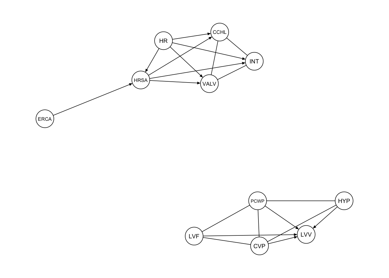
The third procedure creates a partial ancestral graph (PAG) for the observable vertices in the subset-graph with respect to the latent variables in the vertices set \(V \setminus V^{'}\).
PAGs are graphs which are used to represent causal relationships in situations where the exact underlying causal structure is not fully known or observable. In our case we observe the variables in the set \(V^{'}\). Based on the covariance matrix from the observed data in \(V^{'}\) we generate.
Subsetting the dataset according to “subgraph_nodes” selection
alarm_df_subset <- as_tibble(alarm_df) |>
  select(all_of(subgraph_nodes))
Step 1: Compute the correlation matrix for the observed variables contained in alarm_df_subset.
cor_matrix <- cor(alarm_df_subset)Step 2: Provide necessary information for the algorithm to work on.
indepTest <- pcalg::gaussCItest
suffStat <- list(C = cor_matrix, n = 1000)
Step 3: Apply the FCI algorithm to the selected vertices, using the oracle correlation matrix.
normal.pag <- pcalg:: fci(suffStat, indepTest, alpha = 0.05,
                          labels = subgraph_nodes)
Step 4: Plot the resulting PAG (Partial Ancestral Graph).
qgraph(normal.pag@amat, asize=4, edge.color="black", vsize= 5)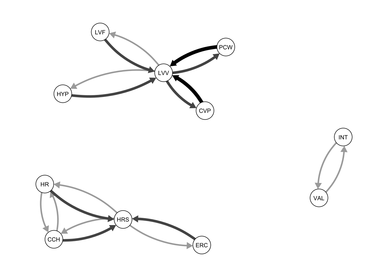
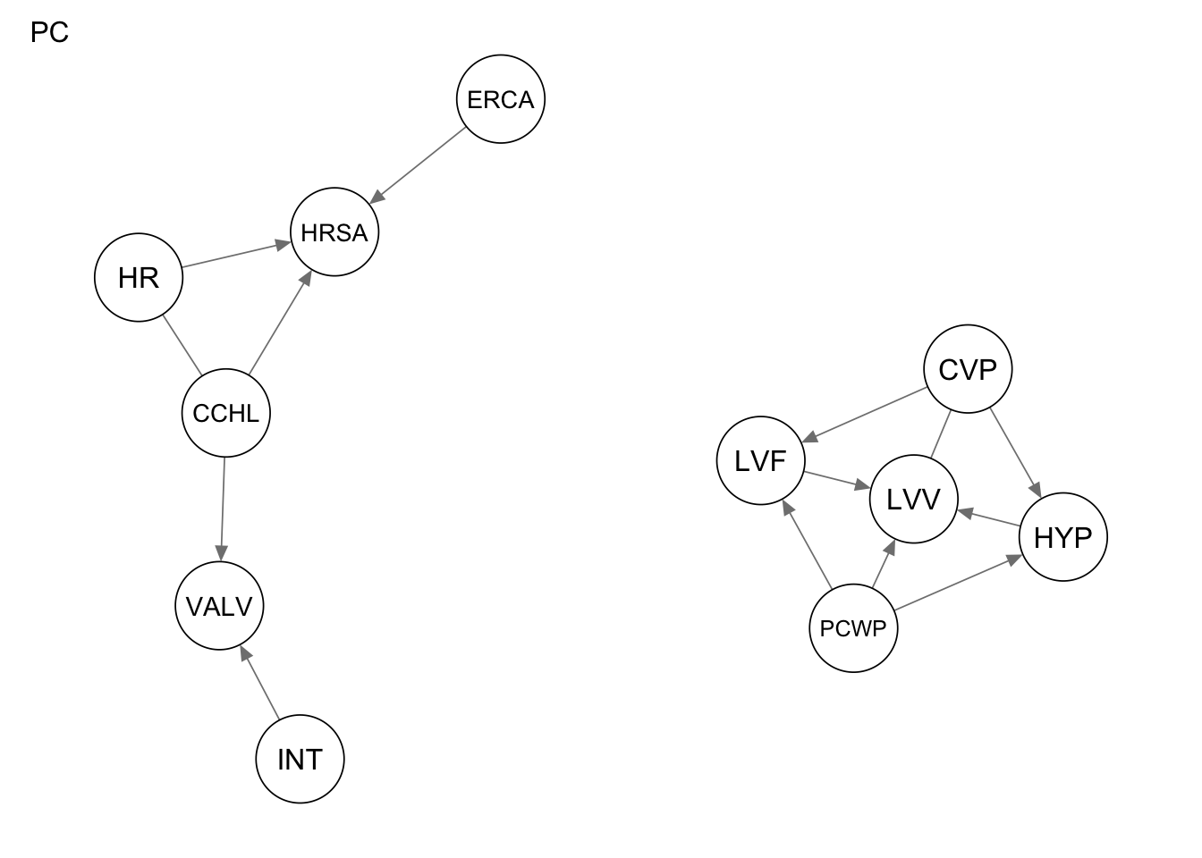
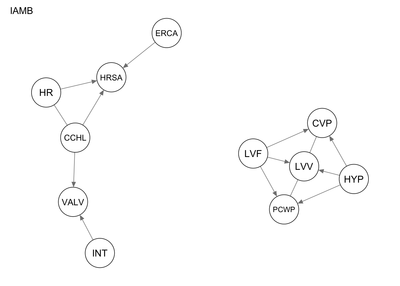
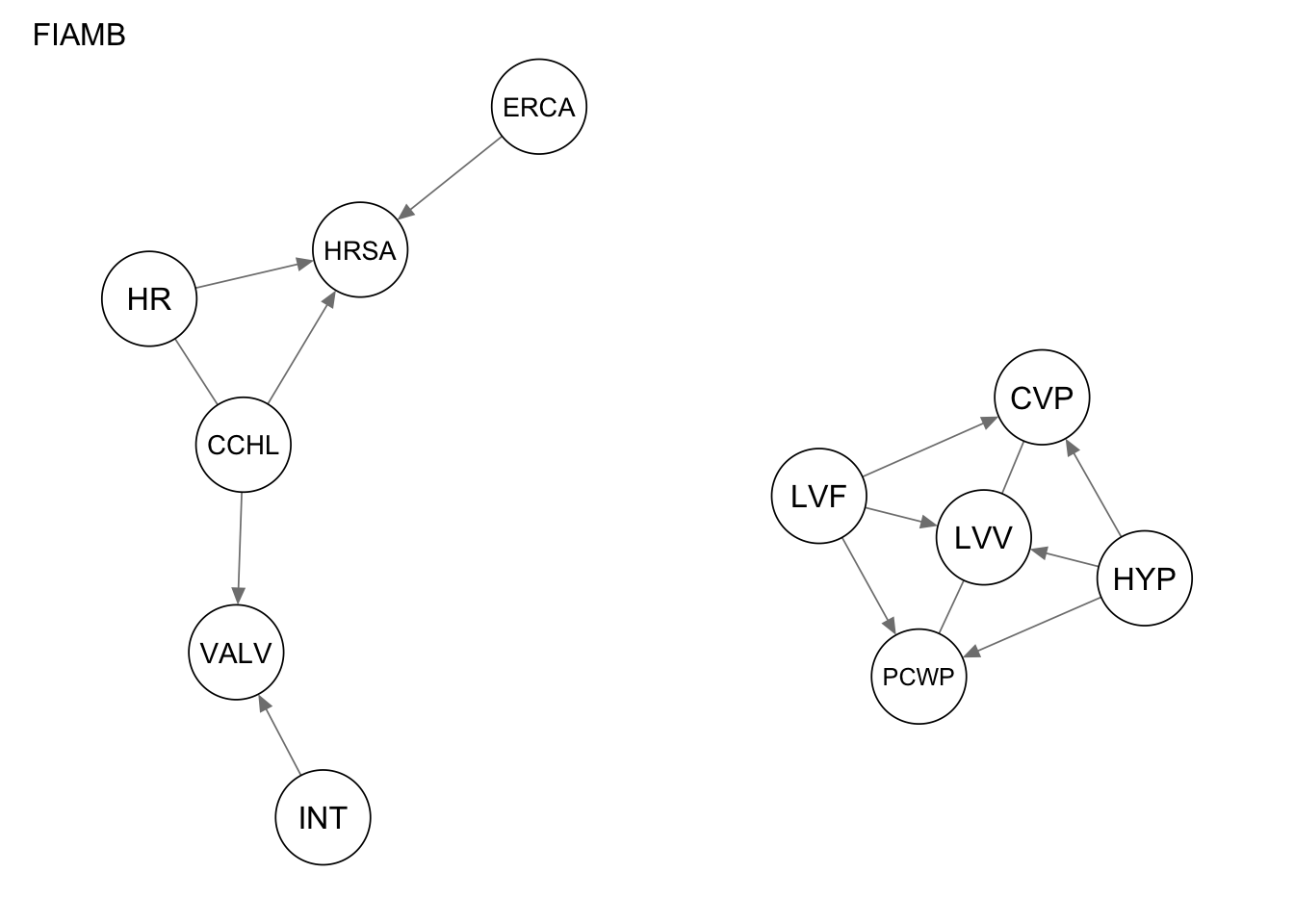
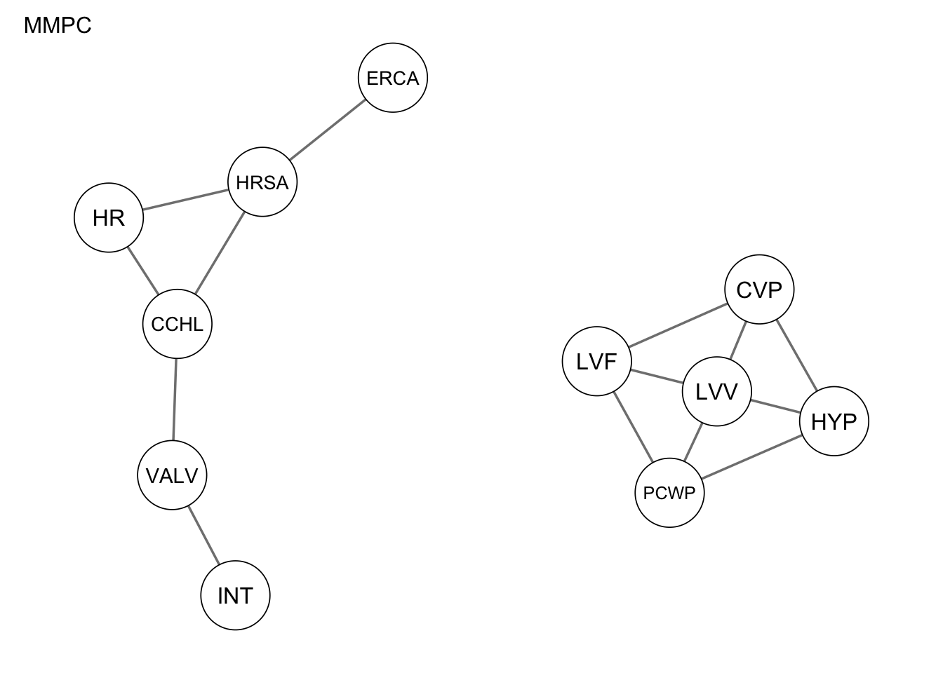
Applying constraint-based algorithms
Res_stable <-pc.stable(alarm_df_subset)
Res_iamb <- iamb(alarm_df_subset)
Res_gs <- gs(alarm_df_subset)
Res_fiamb <- fast.iamb(alarm_df_subset)
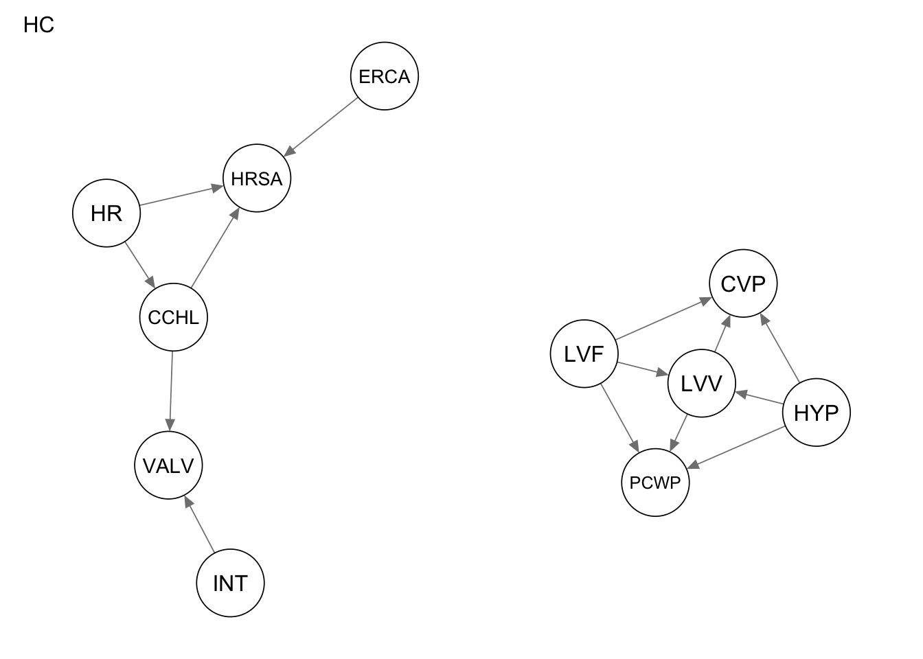
Res_mmpc <- mmpc(alarm_df_subset)Applying score-based algorithms
Res_hc <- hc(alarm_df_subset)
Res_tabu <- tabu(alarm_df_subset)
The resulting subgraphs are shown below.
qgraph(procedure1, title = "Procedure 1")
qgraph(procedure2, title = "Procedure 2")
qgraph(Res_stable, title = "PC")
qgraph(Res_iamb, title = "IAMB")
qgraph(Res_gs, title = "GS")
qgraph(Res_fiamb, title = "FIAMB")
qgraph(Res_mmpc, title = "MMPC")
qgraph(Res_hc, title = "HC")
qgraph(Res_tabu, title = "tabu")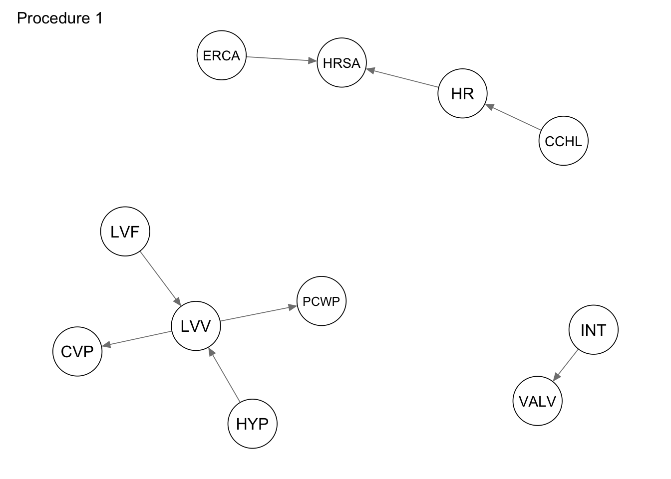


Evaluate the performance by computing the number of true positives, false positives, and false negatives, as well as the structural hamming distance.
measure  <-  function(estim, true){
  result <- matrix(1,4)
  com <- bnlearn::compare(estim, true)
  shd <- bnlearn::shd(estim,true)
  result <- data.frame(
    metric = c("true positives","false positives","false negatives","structural hamming distance"),
    value = c(com$tp, com$fp, com$fn, shd)
  )
  return(result)
}
Metric evaluation for procedure 1
measure(Res_stable, procedure1) metric value
1 true positives 5
2 false positives 3
3 false negatives 9
4 structural hamming distance 9measure(Res_iamb, procedure1) metric value
1 true positives 5
2 false positives 3
3 false negatives 9
4 structural hamming distance 9measure(Res_gs, procedure1) metric value
1 true positives 5
2 false positives 3
3 false negatives 9
4 structural hamming distance 9measure(Res_fiamb, procedure1) metric value
1 true positives 5
2 false positives 3
3 false negatives 9
4 structural hamming distance 9measure(Res_mmpc, procedure1) metric value
1 true positives 0
2 false positives 8
3 false negatives 14
4 structural hamming distance 12measure(Res_hc, procedure1) metric value
1 true positives 7
2 false positives 1
3 false negatives 7
4 structural hamming distance 9measure(Res_tabu, procedure1) metric value
1 true positives 7
2 false positives 1
3 false negatives 7
4 structural hamming distance 9Metric evaluation for procedure 2
measure(Res_stable, procedure2) metric value
1 true positives 5
2 false positives 15
3 false negatives 9
4 structural hamming distance 15measure(Res_iamb, procedure2) metric value
1 true positives 4
2 false positives 16
3 false negatives 10
4 structural hamming distance 16measure(Res_gs, procedure2) metric value
1 true positives 4
2 false positives 16
3 false negatives 10
4 structural hamming distance 16measure(Res_fiamb, procedure2) metric value
1 true positives 4
2 false positives 16
3 false negatives 10
4 structural hamming distance 16measure(Res_mmpc, procedure2) metric value
1 true positives 6
2 false positives 14
3 false negatives 8
4 structural hamming distance 14measure(Res_hc, procedure2) metric value
1 true positives 5
2 false positives 15
3 false negatives 9
4 structural hamming distance 16measure(Res_tabu, procedure2) metric value
1 true positives 5
2 false positives 15
3 false negatives 9
4 structural hamming distance 16source("../../close_environment.R")sessionInfo()R version 4.4.2 (2024-10-31)
Platform: aarch64-apple-darwin20
Running under: macOS 26.2
Matrix products: default
BLAS: /Library/Frameworks/R.framework/Versions/4.4-arm64/Resources/lib/libRblas.0.dylib
LAPACK: /Library/Frameworks/R.framework/Versions/4.4-arm64/Resources/lib/libRlapack.dylib; LAPACK version 3.12.0
locale:
[1] en_US.UTF-8/en_US.UTF-8/en_US.UTF-8/C/en_US.UTF-8/en_US.UTF-8
time zone: Europe/Berlin
tzcode source: internal
attached base packages:
[1] stats graphics grDevices datasets utils methods base
other attached packages:
[1] dplyr_1.1.4 zen4R_0.10.2 huge_1.3.5 pcalg_2.7-12 igraph_2.1.4
[6] qgraph_1.9.8 bnlearn_5.0.2
loaded via a namespace (and not attached):
[1] mnormt_2.1.1 RBGL_1.82.0 pbapply_1.7-2
[4] gridExtra_2.3 fdrtool_1.2.18 rlang_1.1.6
[7] magrittr_2.0.3 clue_0.3-66 compiler_4.4.2
[10] roxygen2_7.3.2 png_0.1-8 vctrs_0.6.5
[13] reshape2_1.4.4 quadprog_1.5-8 stringr_1.5.1
[16] pkgconfig_2.0.3 crayon_1.5.3 fastmap_1.2.0
[19] backports_1.5.0 utf8_1.2.6 pbivnorm_0.6.0
[22] rmarkdown_2.29 tzdb_0.5.0 graph_1.84.1
[25] purrr_1.1.0 bit_4.6.0 xfun_0.52
[28] jsonlite_2.0.0 jpeg_0.1-11 psych_2.5.6
[31] parallel_4.4.2 lavaan_0.6-19 cluster_2.1.8
[34] R6_2.6.1 stringi_1.8.7 RColorBrewer_1.1-3
[37] rdflib_0.2.9 rpart_4.1.24 Rcpp_1.1.0
[40] knitr_1.50 ggm_2.5.1 base64enc_0.1-3
[43] readr_2.1.5 Matrix_1.7-2 nnet_7.3-20
[46] tidyselect_1.2.1 rstudioapi_0.17.1 abind_1.4-8
[49] yaml_2.3.10 codetools_0.2-20 curl_6.4.0
[52] lattice_0.22-6 tibble_3.3.0 plyr_1.8.9
[55] withr_3.0.2 evaluate_1.0.4 foreign_0.8-88
[58] zip_2.3.3 xml2_1.3.8 pillar_1.11.0
[61] BiocManager_1.30.26 checkmate_2.3.2 renv_1.1.4
[64] stats4_4.4.2 generics_0.1.4 vroom_1.6.5
[67] hms_1.1.3 ggplot2_3.5.2 scales_1.4.0
[70] fastICA_1.2-7 gtools_3.9.5 glue_1.8.0
[73] Hmisc_5.2-3 tools_4.4.2 robustbase_0.99-4-1
[76] data.table_1.17.8 XML_3.99-0.18 grid_4.4.2
[79] tidyr_1.3.1 bdsmatrix_1.3-7 colorspace_2.1-1
[82] nlme_3.1-167 sfsmisc_1.1-20 htmlTable_2.4.3
[85] Formula_1.2-5 cli_3.6.5 atom4R_0.3-3
[88] keyring_1.4.1 Rgraphviz_2.50.0 corpcor_1.6.10
[91] glasso_1.11 gtable_0.3.6 DEoptimR_1.1-3-1
[94] digest_0.6.37 BiocGenerics_0.52.0 redland_1.0.17-18
[97] htmlwidgets_1.6.4 farver_2.1.2 htmltools_0.5.8.1
[100] lifecycle_1.0.4 httr_1.4.7 bit64_4.6.0-1
[103] MASS_7.3-64 Citing this Notebook
Please cite ALARM Subgraph Analysis with the following bib item.
@misc{HaugZadorozhnyi2025,
  title = {ALARM Subgraph Analysis},
  author = {Haug, Stephan and Zadorozhnyi, Oleksandr},
  year = {2025}
}
When using the ALARM dataset, please give credit to the original author: Scutari (2010).
Scutari, Marco. 2010. “Learning Bayesian Networks with the Bnlearn r Package.” Journal of Statistical Software 35 (3): 1–22. https://doi.org/10.18637/jss.v035.i03.
Additional Information
License Information: Please follow the above DOI for license information of data and code.
Contact: If you have suggestions, feel free to create an issue or contact the authors (haug@tum.de).