3  SEMID Package for Deciding Identifiability in Linear Causal Models

Author

Affiliation

Nils Sturma

Ecole polytechnique fédérale de Lausanne (EPFL)

Resource	Information
Git + DOI	Git 10.5281/zenodo.17475524
Short Description	The SEMID package offers a number of different functions for deciding global and generic identifiability in linear structural equation models with latent variables. In this notebook, we present its main functionality. We also show how to use easy plug-in estimators if identifiability holds.

3.1 Introduction

This notebook presents the SEMID package that offers a number of different functions for deciding global and generic identifiability in linear structural equation models (SEMs) with latent variables. Each model is defined by a directed graph or by a mixed graph, depending on the modeling assumptions. Identifiability holds if the linear coefficients corresponding to the direct causal effects can be uniquely recovered from the covariance matrix of the observable distribution.

We first load the required packages.

# Used packages, only for information
library(SEMID) # deciding identifiability
library(MASS) # sampling from multivariate normal distribution

3.2 Linear SEMs Given by Mixed Graphs

In linear structural equation models given by mixed graphs, the confounding effects of the latent variables are represented by correlation among noise terms. Let \(G=(V,D,B)\) be a mixed graph, where \(V=\{1, \ldots, p\}\) is a finite set of nodes, \(D\) is a set of directed edges, and \(B\) is a set of bidirected edges. Moreover, let \(X=(X_v)_{v \in V}\) be a random vector that is indexed by the nodes of the graph. We suppose that \(X\) solves the linear equation system \[ X = \Lambda^{\top} X + \varepsilon, \] where \(\varepsilon = (\varepsilon_v)_{v \in V}\) is a vector of noise variables with mean zero and positive definite covariance matrix \(\Omega = (\omega_{vw})\). Two noise variables \(\varepsilon_v\) and \(\varepsilon_w\) are assumed to be uncorrelated whenever there is no bidirected edge in the graph, i.e., in this case it holds that \(\omega_{vw} = 0\). The coefficient matrix \(\Lambda = (\lambda_{vw})\) is sparse according to the bidirected part of the graph, that is, \(\lambda_{vw} = 0\) if the directed edge from \(v\) to \(w\) is not in \(D\). The coefficients \(\lambda_{vw}\) may be interpreted as direct causal effects and are the main objects of interest. Note that if \(I - \Lambda\) is invertible, then the covariance matrix of \(X\) is given by \[ \Sigma := \text{Cov}[X] = (I - \Lambda)^{-\top} \Omega (I - \Lambda)^{-1}. \] Identifiability holds if we can recover the matrix \(\Lambda\) uniquely from a given covariance matrix \(\Sigma\). We differentiate between global and generic identifiability: A mixed graph is said to be globally identifiable, if identifiability holds for all parameter choices. On the other hand, a mixed graph is said to be generically identifiable, if identifiability holds for almost all parameter choices. Note that a graph is generically identifiable if and only if all directed edges are generically identifiable.

In the SEMID package, we represent mixed graphs via the MixedGraph class. The implementation is using the R.oo package by Bengtsson (2003).

Bengtsson, Henrik. 2003. “The R.oo Package - Object-Oriented Programming with References Using Standard R Code.” In Proceedings of the 3rd International Workshop on Distributed Statistical Computing (DSC 2003), edited by Kurt Hornik, Friedrich Leisch, and Achim Zeileis. Vienna, Austria: https://www.r-project.org/conferences/DSC-2003/Proceedings/. https://www.r-project.org/conferences/DSC-2003/Proceedings/Bengtsson.pdf.

# Mixed graphs are specified by their directed adjacency matrix L 
# and bidirected adjacency matrix O.
L <- t(matrix(c(0, 1, 0, 0, 0,
                0, 0, 0, 1, 1,
                0, 0, 0, 1, 0,
                0, 1, 0, 0, 1,
                0, 0, 0, 1, 0), 5, 5))

O <- t(matrix(c(0, 0, 0, 0, 0,
                0, 0, 1, 0, 1,
                0, 0, 0, 1, 0,
                0, 0, 0, 0, 0,
                0, 0, 0, 0, 0), 5, 5)); O<-O+t(O)

# Create the mixed graph object corresponding to L and O
g <- MixedGraph(L, O)

# Plot the mixed graph
g$plot()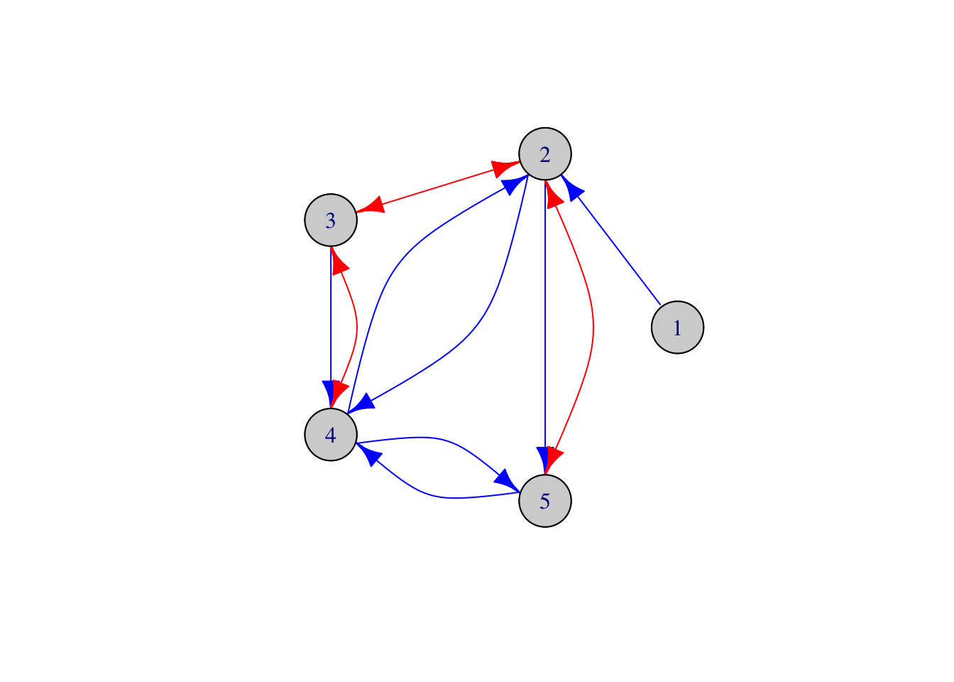

For deciding global identifiability, there exists an ‘if and only if’ graphical criterion developed by Drton, Foygel, and Sullivant (2011). This criterion can be accessed through the function globalID.

Drton, Mathias, Rina Foygel, and Seth Sullivant. 2011. “Global Identifiability of Linear Structural Equation Models.” Ann. Statist. 39 (2): 865–86. https://doi.org/10.1214/10-AOS859.

# Check global identifiability
SEMID::globalID(g)

[1] FALSE

There still do not exist any ‘if and only if’ graphical conditions for testing whether or not a mixed graph is generically identifiable. However, there do exist sufficient and necessary conditions. The SEMID package contains implementations of various sufficient conditions: The half-trek criterion by Foygel, Draisma, and Drton (2012), ancestor decomposition techniques by Drton and Weihs (2016), and the edgewise and determinantal criteria by Weihs et al. (2017).

Drton, Mathias, and Luca Weihs. 2016. “Generic Identifiability of Linear Structural Equation Models by Ancestor Decomposition.” Scand. J. Stat. 43 (4): 1035–45. https://doi.org/10.1111/sjos.12227.

Weihs, Luca, Bill Robinson, Emilie Dufresne, Jennifer Kenkel, Kaie Kubjas Reginald McGee II, McGee II Reginald, Nhan Nguyen, Elina Robeva, and Mathias Drton. 2017. “Determinantal Generalizations of Instrumental Variables.” J. Causal Inference 6 (1). https://doi.org/10.1515/jci-2017-0009.

# Check generic identifiability using different criteria
SEMID::htcID(g)

Call: SEMID::htcID(mixedGraph = g)

Mixed Graph Info.
# nodes: 5 
# dir. edges: 7 
# bi. edges: 3 

Generic Identifiability Summary
# dir. edges shown gen. identifiable: 2 
# bi. edges shown gen. identifiable: 0 

Generically identifiable dir. edges:
2->5, 4->5 

Generically identifiable bi. edges:
None

SEMID::ancestralID(g)

Call: SEMID::ancestralID(mixedGraph = g)

Mixed Graph Info.
# nodes: 5 
# dir. edges: 7 
# bi. edges: 3 

Generic Identifiability Summary
# dir. edges shown gen. identifiable: 2 
# bi. edges shown gen. identifiable: 0 

Generically identifiable dir. edges:
2->5, 4->5 

Generically identifiable bi. edges:
None

SEMID::edgewiseID(g)

Call: SEMID::edgewiseID(mixedGraph = g)

Mixed Graph Info.
# nodes: 5 
# dir. edges: 7 
# bi. edges: 3 

Generic Identifiability Summary
# dir. edges shown gen. identifiable: 4 
# bi. edges shown gen. identifiable: 0 

Generically identifiable dir. edges:
2->4, 5->4, 2->5, 4->5 

Generically identifiable bi. edges:
None

SEMID::edgewiseTSID(g)

Call: SEMID::edgewiseTSID(mixedGraph = g)

Mixed Graph Info.
# nodes: 5 
# dir. edges: 7 
# bi. edges: 3 

Generic Identifiability Summary
# dir. edges shown gen. identifiable: 4 
# bi. edges shown gen. identifiable: 0 

Generically identifiable dir. edges:
2->4, 5->4, 2->5, 4->5 

Generically identifiable bi. edges:
None

Note that, by default, all strategies first apply a Tian decomposition and then check identifiability on each of the components. This yields faster computations as described in Section 8 of Foygel, Draisma, and Drton (2012). It is also possible to apply different identification strategies repeatedly until no further edges can be identified. This is possible via the function generalGenericID.

# Check generic identifiability by repeatedly applying different criteria
SEMID::generalGenericID(mixedGraph = g, 
                 idStepFunctions = list(htcIdentifyStep,
                                        ancestralIdentifyStep, 
                                        edgewiseIdentifyStep, 
                                        trekSeparationIdentifyStep), 
                 tianDecompose = TRUE)

Call: SEMID::generalGenericID(mixedGraph = g, idStepFunctions = list(htcIdentifyStep, 
    ancestralIdentifyStep, edgewiseIdentifyStep, trekSeparationIdentifyStep), 
    tianDecompose = TRUE)

Mixed Graph Info.
# nodes: 5 
# dir. edges: 7 
# bi. edges: 3 

Generic Identifiability Summary
# dir. edges shown gen. identifiable: 4 
# bi. edges shown gen. identifiable: 0 

Generically identifiable dir. edges:
2->4, 5->4, 2->5, 4->5 

Generically identifiable bi. edges:
None

In this example, we do not get additional edges certified to be generically identifiability. Therefore, we check the necessary condition from Foygel, Draisma, and Drton (2012) for generic identifiability of the whole graph, which is also implemented in SEMID.

Foygel, Rina, Jan Draisma, and Mathias Drton. 2012. “Half-Trek Criterion for Generic Identifiability of Linear Structural Equation Models.” Ann. Statist. 40 (3): 1682–1713. https://doi.org/10.1214/12-AOS1012.

# Check necessary condition for generic identifiability 
SEMID::graphID.nonHtcID(g$L(), g$O())

[1] TRUE

This means that the given graph is infinite-to-one and, in particular, not generically identifiable.

3.3 Linear SEMs Given by Latent-Factor Graphs

The approach to model confounding via correlation is only effective when the confounding is sparse and effects only small subsets of the observed variables. There also exist criteria for checking identifiability in unprojected models, where some latent variables may also have dense effects on many or even all of the observables. One approach is the Latent-Factor Half-Trek Criterion by Barber et al. (2022), which operates on directed graphs with explicit latent nodes. However, the latent variables are restricted to be source nodes of the graph. Let \(V\) be a finite set of observed nodes and let \(\mathcal{L}\) be a disjoint, finite set of latent nodes. A latent-factor graph is a direct graph \(G=(V \cup \mathcal{L},D)\) in which all latent variables are source nodes. Let \(X=(X_v)_{v \in V}\) be an observed random vector, and let \(L = (L_h)_{h \in \mathcal{L}}\) be a latent random vector. We suppose that all variables are related via the equation system \[ X = \Lambda^{\top} X + \Gamma^{\top} L + \varepsilon, \] where the vector \(\varepsilon\) contains independent noise variables with mean zero and diagonal, positive definite covariance matrix \(\Omega_{\text{diag}}\). Both coefficient matrices \(\Lambda=(\lambda_{vw})\) and \(\Gamma=(\gamma_{hv})\) are sparse according to the graph, that is, \(\lambda_{vw} = 0\) if the directed edge from the observed node \(v\) to the observed node \(w\) is not in \(D\), and \(\gamma_{hv} = 0\) if the directed edge from the latent node \(h\) to the observed node \(v\) is not in \(D\). Our main objects of interest are again the direct causal effects \(\lambda_{vw}\) between the observed variables. If \(I - \Lambda\) is invertible, the covariance matrix of \(X\) is given by \[ \Sigma := \text{Cov}[X] = (I - \Lambda)^{-\top} (\Gamma^{\top} \Gamma + \Omega_{\text{diag}}) (I - \Lambda)^{-1}. \] Similar as for mixed graphs, we say that a latent-factor graph is generically identifiable if we can uniquely recover all direct causal effects from the covariance matrix for almost all parameter choices.

In the SEMID package, we represent latent-factor graphs via the LatentDigraph class.

# Latent digraphs are specified by their directed adjacency matrix L and 
# their vectors of observed and latent nodes
L <- t(matrix(c(0, 1, 0, 0, 0, 0,
                0, 0, 1, 0, 0, 0,
                0, 0, 0, 0, 0, 0,
                0, 0, 0, 0, 1, 0,
                0, 0, 0, 0, 0, 0,
                1, 1, 1, 1, 1, 0), 6, 6))
observedNodes <- seq(1,5)
latentNodes <- c(6)

# Create the latent digraph object
g <- SEMID::LatentDigraph(L, observedNodes, latentNodes)

# Plot the mixed graph
g$plot()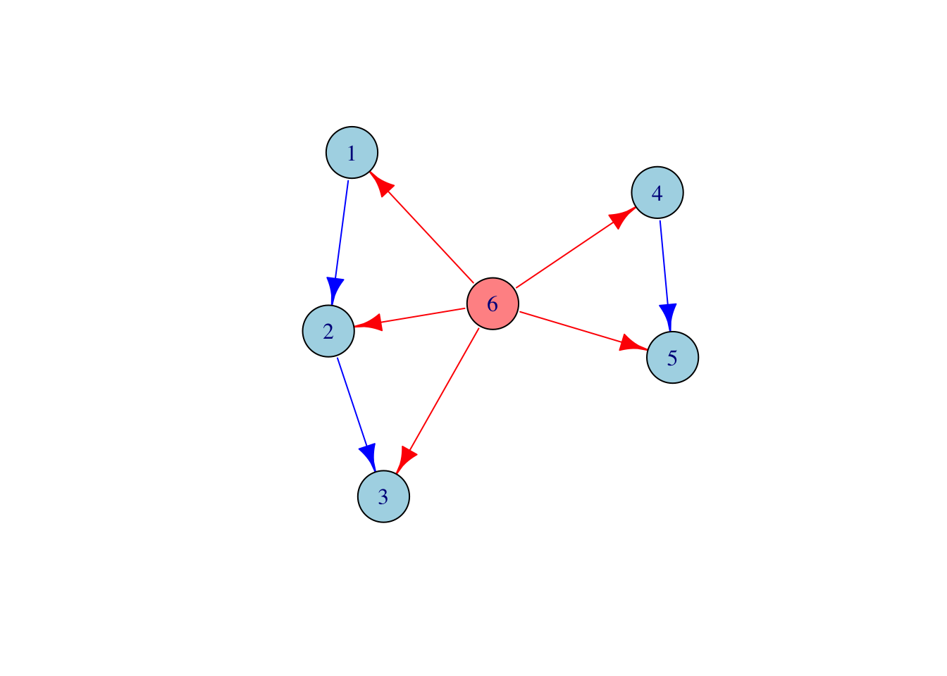

The latent-factor half-trek criterion by Barber et al. (2022) is a sufficient condition for generic identifiability. The criterion can be accessed through the function lfhtcID.

# Check generic identifiability of the latent-factor graph
SEMID::lfhtcID(g)

Call: SEMID::lfhtcID(graph = g)

Latent Digraph Info
# observed nodes: 5 
# latent nodes: 1 
# total nr. of edges between observed nodes: 3 

Generic Identifiability Summary
# nr. of edges between observed nodes shown gen. identifiable: 3 
# gen. identifiable edges: 1->2, 2->3, 4->5 

Note that the corresponding mixed graph obtained from a latent projection is not identifiable (see Section 4 in Barber et al. (2022)).

Barber, Rina Foygel, Mathias Drton, Nils Sturma, and Luca Weihs. 2022. “Half-trek criterion for identifiability of latent variable models.” Ann. Statist. 50 (6): 3174–96. https://doi.org/10.1214/22-AOS2221.

# Get a mixed graph via latent projection
gMixed <- g$getMixedGraph()
gMixed$plot()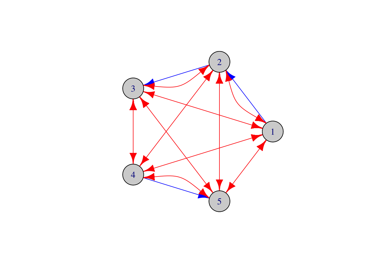

# Check the original half-trek criterion on the mixed graph
SEMID::htcID(gMixed)

Call: SEMID::htcID(mixedGraph = gMixed)

Mixed Graph Info.
# nodes: 5 
# dir. edges: 3 
# bi. edges: 10 

Generic Identifiability Summary
# dir. edges shown gen. identifiable: 0 
# bi. edges shown gen. identifiable: 0 

Generically identifiable dir. edges:
None

Generically identifiable bi. edges:
None

3.4 Estimating Direct Causal Effects

If a graph is generically identifiable, we can use the identification formulas to obtain estimators of the direct causal effects. We demonstrate this with the example of the following mixed graph:

# Define Mixed Graph
L <- t(matrix(c(0, 1, 0, 0, 0,
                0, 0, 0, 0, 0,
                0, 0, 0, 1, 0,
                0, 0, 0, 0, 1,
                0, 0, 0, 0, 0), 5, 5))

O <- t(matrix(c(0, 0, 1, 1, 0,
                0, 0, 0, 1, 1,
                0, 0, 0, 0, 0,
                0, 0, 0, 0, 0,
                0, 0, 0, 0, 0), 5, 5)); O<-O+t(O)

# Create the mixed graph object corresponding to L and O
g <- MixedGraph(L, O)

# Plot the mixed graph
g$plot()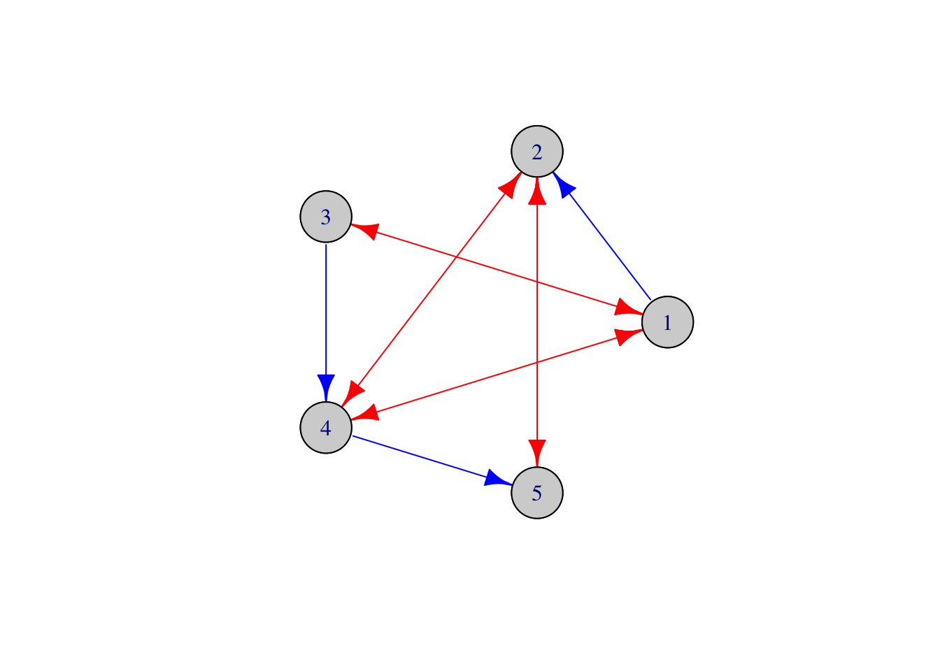

First, we verify that the graph is generically identifiable using the half-trek criterion.

res <- htcID(g)
res

Call: htcID(mixedGraph = g)

Mixed Graph Info.
# nodes: 5 
# dir. edges: 3 
# bi. edges: 4 

Generic Identifiability Summary
# dir. edges shown gen. identifiable: 3 
# bi. edges shown gen. identifiable: 4 

Generically identifiable dir. edges:
1->2, 3->4, 4->5 

Generically identifiable bi. edges:
1<->3, 1<->4, 2<->4, 2<->5 

Next, we randomly choose parameters and sample from a normal distribution that lies in the linear structural equation model given by the above graph.

# Create random parameter matrices that preserve the zero structure
# Lambda
Lambda <- matrix(0, nrow=nrow(L), ncol=ncol(L))
maskL <- (L != 0)
nObsEdges <- sum(maskL)
Lambda[maskL] <- runif(nObsEdges, min = -1, max = 1)
Lambda

     [,1]       [,2] [,3]       [,4]      [,5]
[1,]    0 -0.1943715    0  0.0000000 0.0000000
[2,]    0  0.0000000    0  0.0000000 0.0000000
[3,]    0  0.0000000    0 -0.5552419 0.0000000
[4,]    0  0.0000000    0  0.0000000 0.5606517
[5,]    0  0.0000000    0  0.0000000 0.0000000

# Omega
Omega<- matrix(0, nrow=nrow(O), ncol=ncol(O))
upper_idx <- which(upper.tri(O) & O != 0, arr.ind = TRUE)
k_upper <- nrow(upper_idx)
if (k_upper > 0) {
  vals <- runif(k_upper, min = -1, max = 1)
  for (i in seq_len(k_upper)) {
    Omega[upper_idx[i, "row"], upper_idx[i, "col"]] <- vals[i]
    Omega[upper_idx[i, "col"], upper_idx[i, "row"]] <- vals[i]
  }
}
diag(Omega) <- runif(nrow(O), min = 2, max = 3)
Omega

           [,1]       [,2]       [,3]       [,4]       [,5]
[1,]  2.6687726  0.0000000 -0.3688529 -0.2027899  0.0000000
[2,]  0.0000000  2.9093706  0.0000000 -0.9783949 -0.8698205
[3,] -0.3688529  0.0000000  2.6198380  0.0000000  0.0000000
[4,] -0.2027899 -0.9783949  0.0000000  2.7744870  0.0000000
[5,]  0.0000000 -0.8698205  0.0000000  0.0000000  2.2380906

# Calculate the covariance matrix
id <- diag(nrow(O))
Sigma <- solve(t(id - Lambda)) %*% Omega %*% solve(id - Lambda)
Sigma

             [,1]        [,2]        [,3]         [,4]         [,5]
[1,]  2.668772638 -0.51873329 -0.36885289  0.002012706  0.001128427
[2,] -0.518733289  3.01019754  0.07169448 -0.978786083 -1.418578582
[3,] -0.368852891  0.07169448  2.61983797 -1.454643867 -0.815548594
[4,]  0.002012706 -0.97878608 -1.45464387  3.582166267  2.008347699
[5,]  0.001128427 -1.41857858 -0.81554859  2.008347699  3.364074206

# For our example, we generate data from N(0, Sigma).
# Number of samples
n <- 1000

# Mean vector (zero)
mu <- rep(0, ncol(Sigma))

# Draw samples
X <- mvrnorm(n = n, mu = mu, Sigma = Sigma)

# Compute sample covariance
Sigma_hat <- cov(X)

Finally, we estimate the coefficient matrices \(\Lambda\) and \(\Omega\). The output of the htcIDfunction contains the identifying formulas, where we plug in the sample covariance.

estimates <- res$identifier(Sigma_hat)
estimates$Lambda

     [,1]       [,2] [,3]       [,4]     [,5]
[1,]    0 -0.1847531    0  0.0000000 0.000000
[2,]    0  0.0000000    0  0.0000000 0.000000
[3,]    0  0.0000000    0 -0.5548468 0.000000
[4,]    0  0.0000000    0  0.0000000 1.470755
[5,]    0  0.0000000    0  0.0000000 0.000000

estimates$Omega

           [,1]       [,2]       [,3]       [,4]       [,5]
[1,]  2.6051985 -0.0957324 -0.4309686 -0.1923925  0.0000000
[2,] -0.0957324  3.0290713  0.0000000 -0.9669484 -0.1882484
[3,] -0.4309686  0.0000000  2.7249882  0.0000000  1.3707504
[4,] -0.1923925 -0.9669484  0.0000000  2.8223279 -2.5395634
[5,]  0.0000000 -0.1882484  1.3707504 -2.5395634  5.4988662

Citing This Notebook

Please cite this notebook with the following bib item.

@misc{SEMIDnotebook
  title={SEMID Package for Deciding Identifiability in Linear Causal Models},
  author={Sturma, Nils},
  howpublished={Web Notebook},
  year={2025},
  url={https://st-mardi.quarto.pub/gmci/chapters/notebook_gallery/notebooks/GMCI-notebook-SEMID/notebook.html}
}

Additional Information

License Information: Please follow the above DOI for license information of data and code.

Contact: If you have suggestions, feel free to create an issue or contact the author (nils.sturma@epfl.ch).